OrionSummerInternship-2023
Orion Summer Internship (House Price Prediction Model)
Kaustubh S Nair 2023-06-30
- 🎯The AMES (Advanced Estate Management System)
- 🎯PRE-PROCESSING & EDA :
- Columns with NO Missing_Values
- Target:SalePrie
- MSSubClass
- LotFrontage
- LotArea
- YearBuilt
- YearRemodAdd
- YearRemodAdd vs YearBuilt
- MasVnrArea
- BsmtFinSF1–
- BsmtFinSF2: Type 2 finished square feet
- TotalBsmtSF: Total square feet of basement
- GrLivArea: Above grade (ground) living area square feet
- FullBath: Full bathrooms above grade
- BedroomAbvGr: Bedrooms above grade
- KitchenAbvGr: Kitchens above grade
- TotRmsAbvGrd: Total rooms above grade (does not include bathrooms)
- Fireplaces: Number of fireplaces
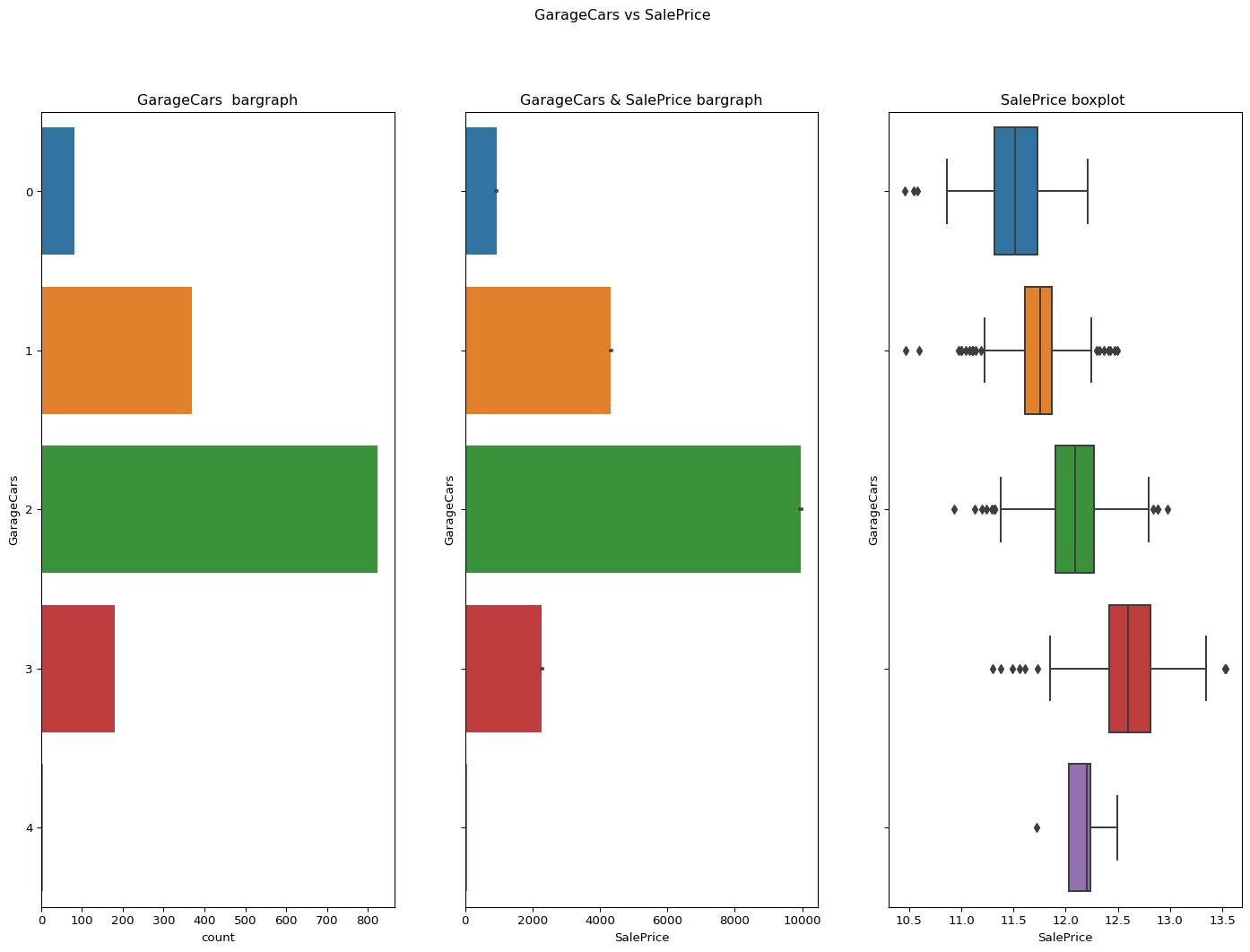
- GarageCars: Size of garage in car capacity
- GarageArea: Size of garage in square feet
- garagecars vs garage area
- OpenPorchSF: Open porch area in square feet(best)
- ScreenPorch: Screen porch area in square feet
- current age of the buildings according to the YearRemodAdd
- Age of the building acc to the yearsold
- garage year built
- 🎯TRAINING AND EVALUATION :
- Select the variables that are Nominal from var_dsc
- Select the variables that are Ordinal from var_dsc
- Select the variables that are Continuous from var_dsc
- Creating arguments for the function to be used
- Dropping the columns with the most missing ratio
- Applying labelencoding , one hot encoding and log tranfromation on the above generated lists
- Splitting the data
- MODEL 1 :
- MODEL 2 :
- ➡️CONCLUSION :
🎯The AMES (Advanced Estate Management System)
House Prediction Regression Model is a machine learning-based system designed to accurately predict house prices. The model leverages regression algorithms and advanced data analysis techniques to estimate the monetary value of residential properties based on a variety of input features. By analyzing historical data and learning from patterns, the AEMS model aims to provide reliable and precise predictions, facilitating informed decision-making in the real estate industry.The model incorporates various stages of data preprocessing and feature engineering to handle missing values, outliers, and transform variables into a suitable format for regression analysis. Techniques such as log transformation, one-hot encoding, and label encoding are applied to ensure the optimal representation of the data. The model also employs advanced regression algorithms, such as linear regression, decision trees, random forests, or gradient boosting, to capture complex relationships and accurately estimate house prices.
Code
``` python import os from dotenv import load_dotenv load_dotenv() # take environment variables from .env. #ROOT_DIR1 = os.environ.get("ROOT_DIR") #print(ROOT_DIR1) ROOT_DIR = os.environ.get("ROOT_DIR2") ```Code
``` python import os os.chdir(ROOT_DIR) import numpy as np import pandas as pd import seaborn as sb from sklearn.preprocessing import LabelEncoder from src.util import catgvssale,contvssale,contvscont,check_column_skewness,remove_skewness,plot_contv,remove_ngskewness,log_transform_continuous,one_hot_encode_nominal,label_encode_dataset,preprocess_dataset from datetime import datetime df = pd.read_csv( "data/raw/train.csv") temp_df=df ```🎯PRE-PROCESSING & EDA :
EDA (Exploratory Data Analysis) and preprocessing play crucial roles in the development of the AEMS House Prediction Regression Model. These stages involve thorough analysis, cleaning, and transformation of the dataset to ensure optimal data quality and feature representation. Analyze the distribution of numerical features and address skewness or non-normality by applying transformations like log transformation.Convert categorical variables into numerical representations using one-hot encoding or label encoding techniques, depending on the nature and cardinality of the variables.
Code
``` python numerics =['int16','int32','int64','float16','float32','float64'] numcol = df.select_dtypes(include=numerics) len(numcol) numcol ```1460 rows × 38 columns
Code
``` python missingper = df.isna().sum().sort_values(ascending=False)/len(df) missingper.head(10) miss_col = missingper[missingper!=0] miss_col miss_col.head(19) ```PoolQC 0.995205
MiscFeature 0.963014
Alley 0.937671
Fence 0.807534
MasVnrType 0.597260
FireplaceQu 0.472603
LotFrontage 0.177397
GarageYrBlt 0.055479
GarageCond 0.055479
GarageType 0.055479
GarageFinish 0.055479
GarageQual 0.055479
BsmtFinType2 0.026027
BsmtExposure 0.026027
BsmtQual 0.025342
BsmtCond 0.025342
BsmtFinType1 0.025342
MasVnrArea 0.005479
Electrical 0.000685
dtype: float64
Columns with NO Missing_Values
Code
``` python nomiss_col = missingper[missingper == 0] nomiss_col nomiss_col.info() nomiss_col.head(15) ```<class 'pandas.core.series.Series'>
Index: 62 entries, Id to SalePrice
Series name: None
Non-Null Count Dtype
-------------- -----
62 non-null float64
dtypes: float64(1)
memory usage: 992.0+ bytes
Id 0.0
Functional 0.0
Fireplaces 0.0
KitchenQual 0.0
KitchenAbvGr 0.0
BedroomAbvGr 0.0
HalfBath 0.0
FullBath 0.0
BsmtHalfBath 0.0
TotRmsAbvGrd 0.0
GarageCars 0.0
GrLivArea 0.0
GarageArea 0.0
PavedDrive 0.0
WoodDeckSF 0.0
dtype: float64
Target:SalePrie
Code
``` python #plot_contv(contvar="SalePrice",df=df) remove_skewness(df,"SalePrice") check_column_skewness(df,"SalePrice") plot_contv(contvar="SalePrice",df=df) ```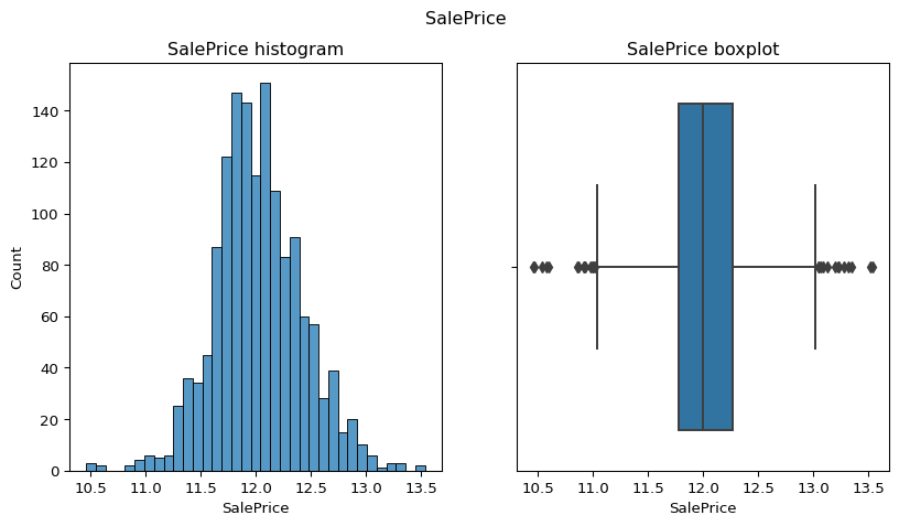
MSSubClass
Code
``` python catgvssale(catgvar="MSSubClass",df=df) check_column_skewness(df,"MSSubClass") ```1.4076567471495591
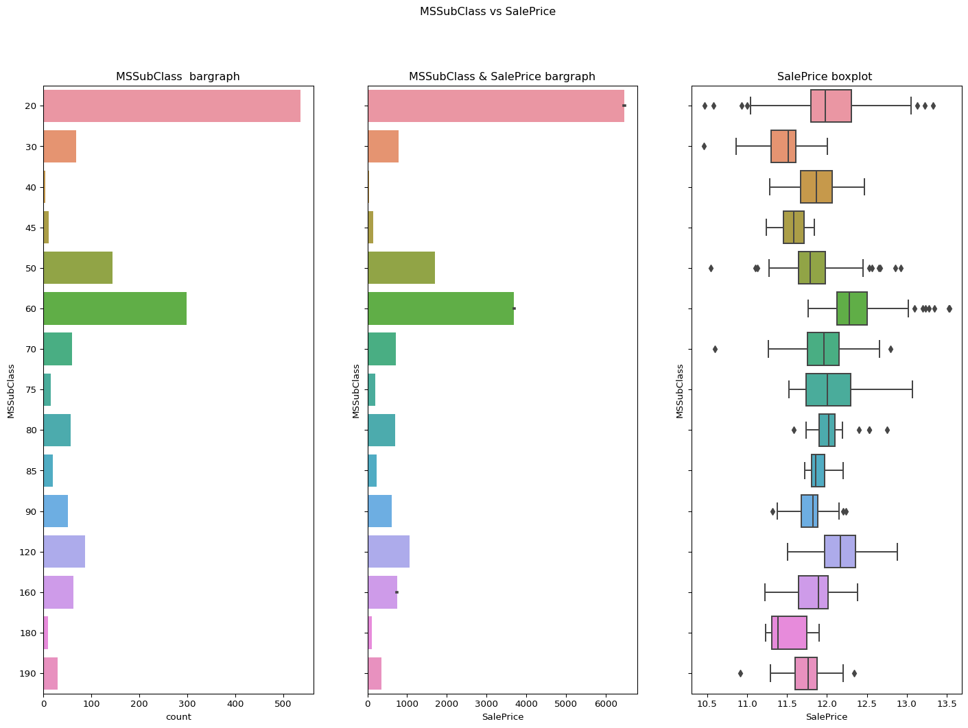
LotFrontage
Checking the skewness of a temporary df which does not include the values of the column LotFrontage which has value 0 and plotting it against the salePrice to check whether it is suitable for the model or not.
Skewness before log transform is 2.1635691423248837.
Now removing the skewness and checking the value againa and plotting it again to see the difference.
Skewness atfer log transform = -0.7287278423055492
Code
``` python temp_df = df.loc[df['LotFrontage']!=0] remove_skewness(temp_df,"LotFrontage") check_column_skewness(temp_df,"LotFrontage") contvssale(contvar="LotFrontage",df=temp_df) ```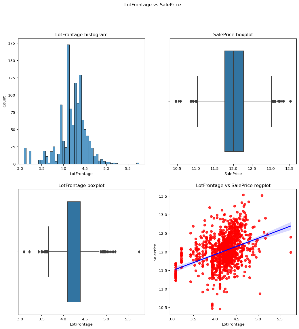
LotArea
Skewness = -0.1374044.
The value is acceptable as it has already been transformed using the log transformation.
Code
``` python remove_skewness(temp_df,"LotArea") contvssale(contvar="LotArea",df=temp_df) ```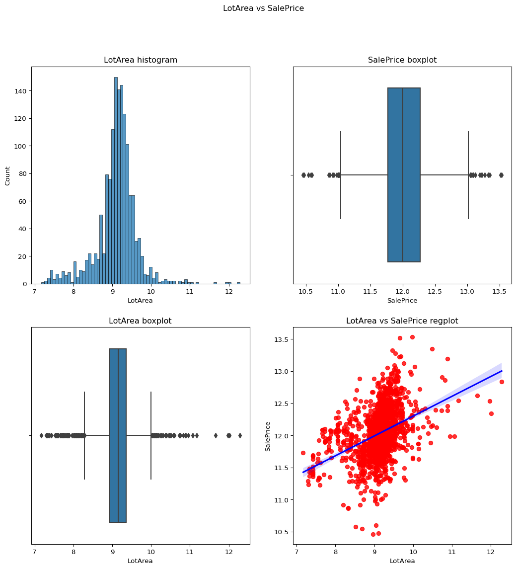
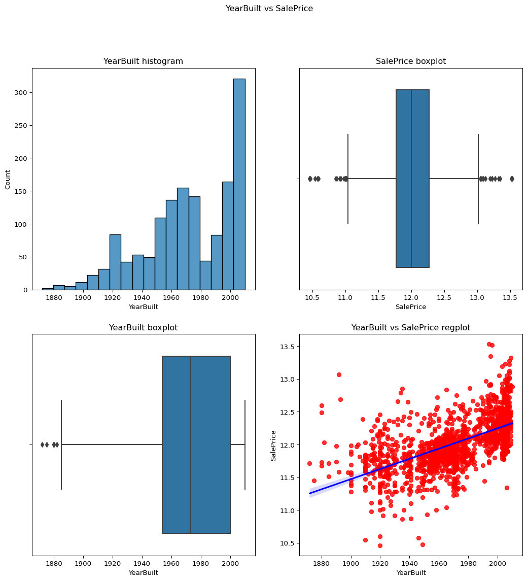
YearBuilt
Skewness = -0.6134611.
As the skewness of the column is already less than 1 there is no need to apply the log transformation.
Code
``` python contvssale(contvar="YearBuilt",df=temp_df) check_column_skewness(temp_df,"YearBuilt") ```-0.613461172488183
YearRemodAdd
Skewness=-0.503562002.
As from the below countplot, boxplot and regplot we can see that this data is not skewed.
Code
``` python contvssale(contvar="YearRemodAdd",df=df) ```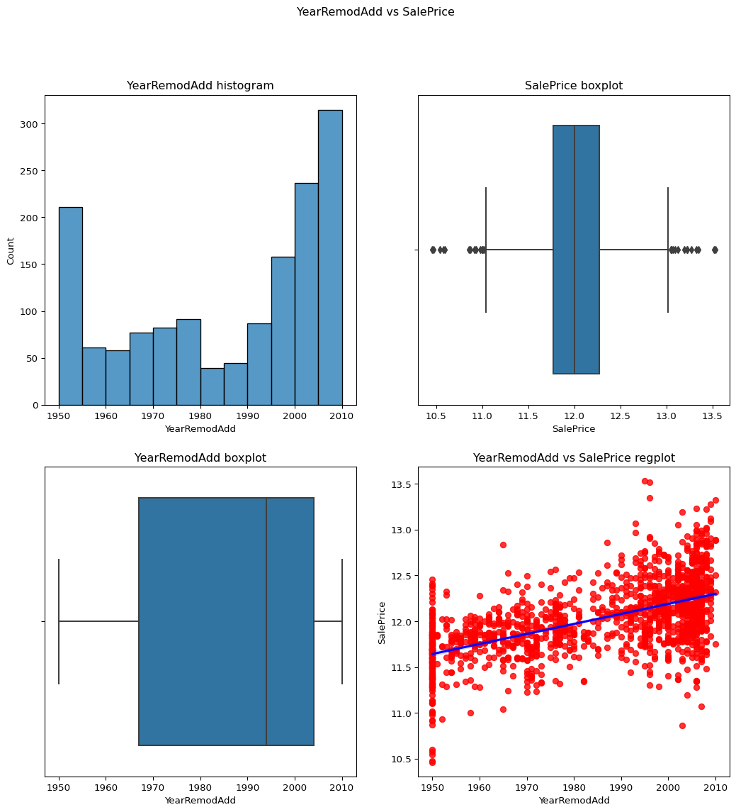
YearRemodAdd vs YearBuilt
Code
``` python contvscont(contvar="YearBuilt",df=df,tarvar="YearRemodAdd") ```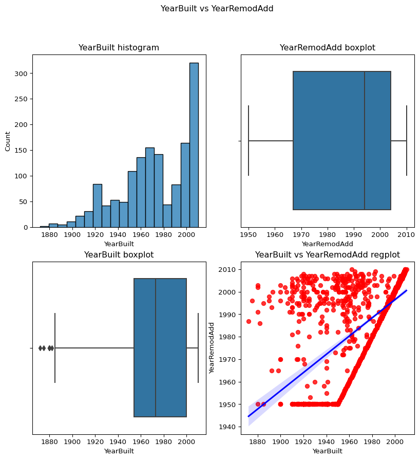
MasVnrArea
Skewness = 2.677616.
From the below graph we can see that this data is a little positively skewed so we can apply here log transformation.
Skewness after = 0.50353171.
Code
``` python op = remove_skewness(df,"MasVnrArea") check_column_skewness(df,"MasVnrArea") contvssale(contvar="MasVnrArea",df=df) ```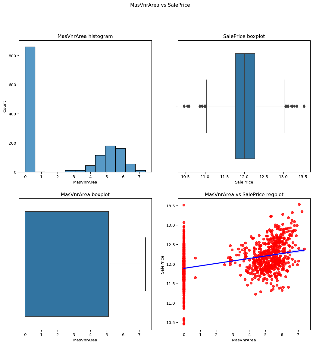
BsmtFinSF1–
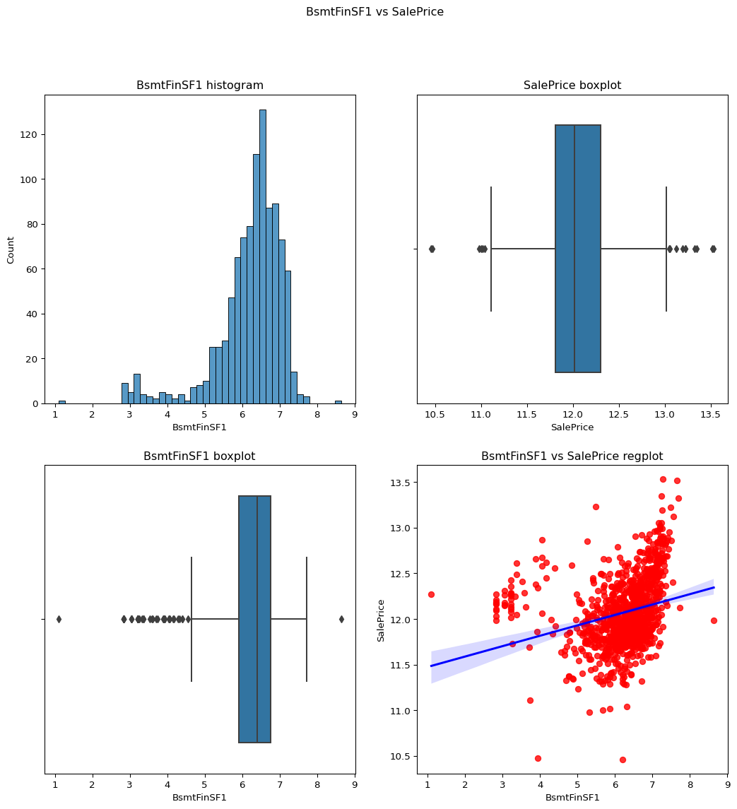
Skewness = 1.685503071910789.
From the regression plot as well as boxplot we can say that this data is slightly skewed as it has more confidence in the regression plot.
Skewness = -0.618409817855514.
Code
``` python remove_skewness(df,"BsmtFinSF1") check_column_skewness(df,"BsmtFinSF1") temp_df = df.loc[df['BsmtFinSF1']!=0] contvssale(contvar="BsmtFinSF1",df=temp_df) check_column_skewness(temp_df,"BsmtFinSF1") ```-1.8212926673745269
BsmtFinSF2: Type 2 finished square feet
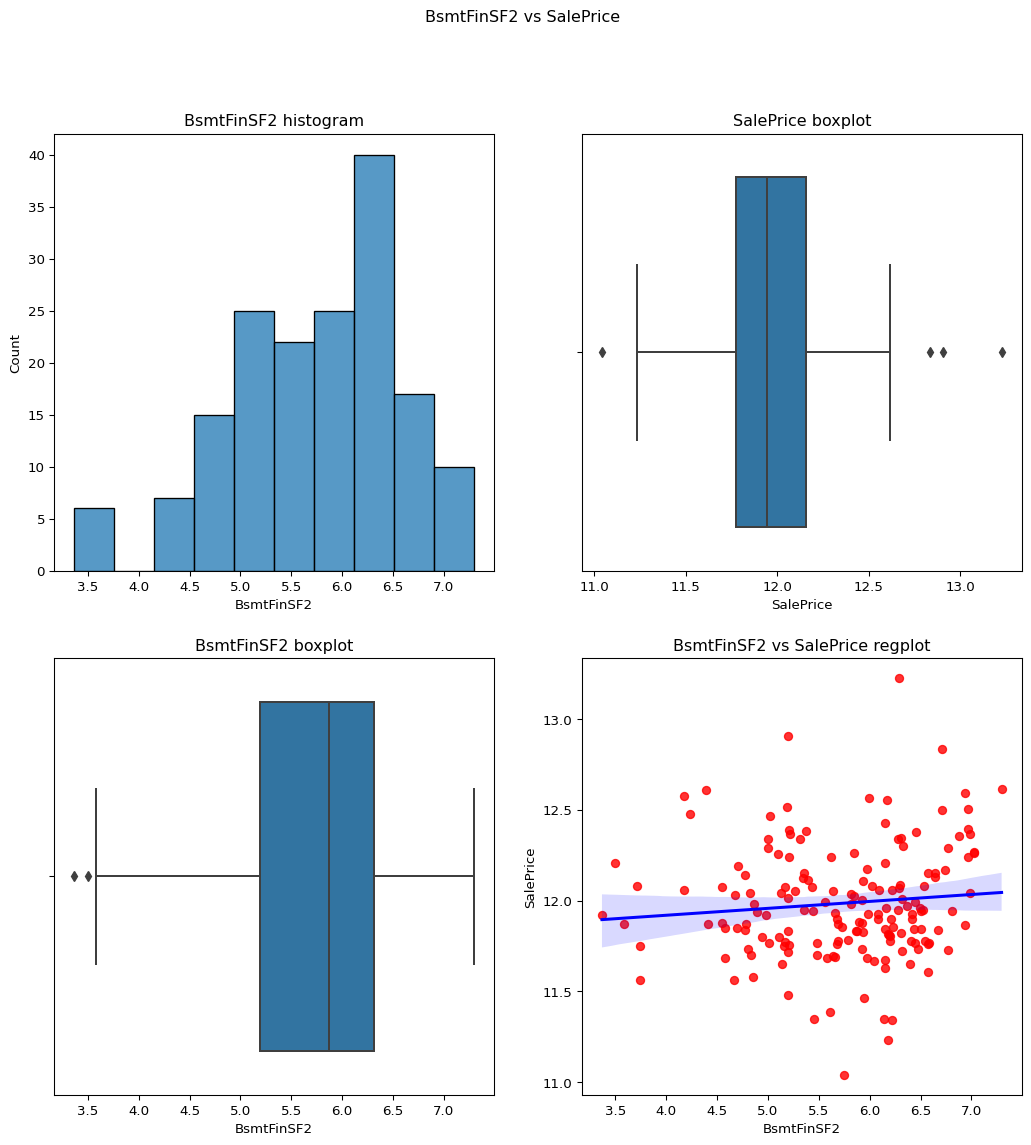
Skewness = 4.255261108933303.
The data is positively skewed and may impact our model so we apply log transform. skewness = 2.434961825856814. After removing the 0 values we get the column with skewness which is less than 1. skewness = 0.9942372017307054
Code
``` python remove_skewness(df,"BsmtFinSF2") check_column_skewness(df,"BsmtFinSF2") temp_df = df.loc[df['BsmtFinSF2']!=0] contvssale(contvar="BsmtFinSF2",df=temp_df) check_column_skewness(temp_df,"BsmtFinSF2") ```-0.5937670428573839
TotalBsmtSF: Total square feet of basement
skewness = 1.5242545490627664
Code
``` python contvssale(contvar="TotalBsmtSF",df=df) ```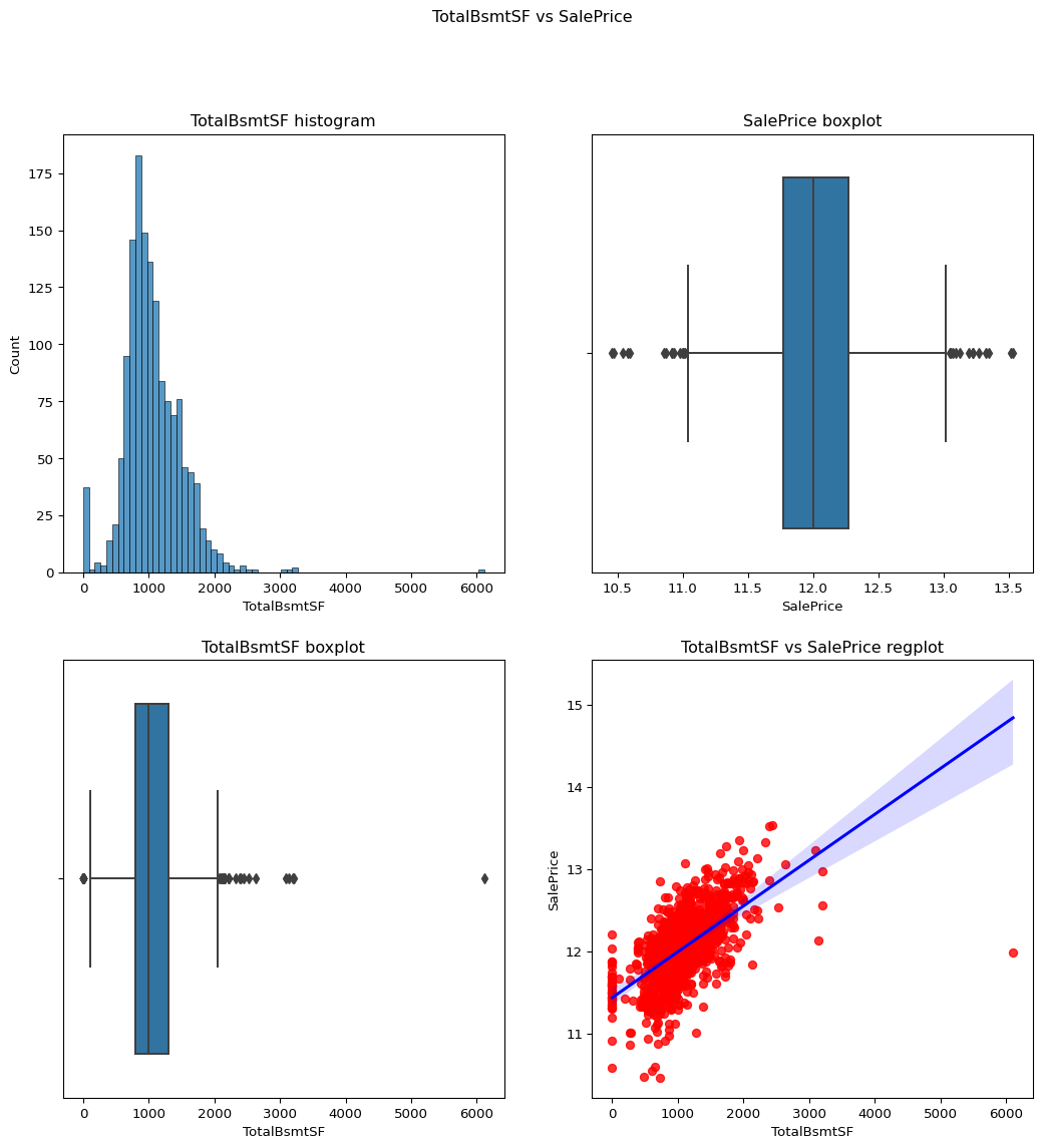
GrLivArea: Above grade (ground) living area square feet
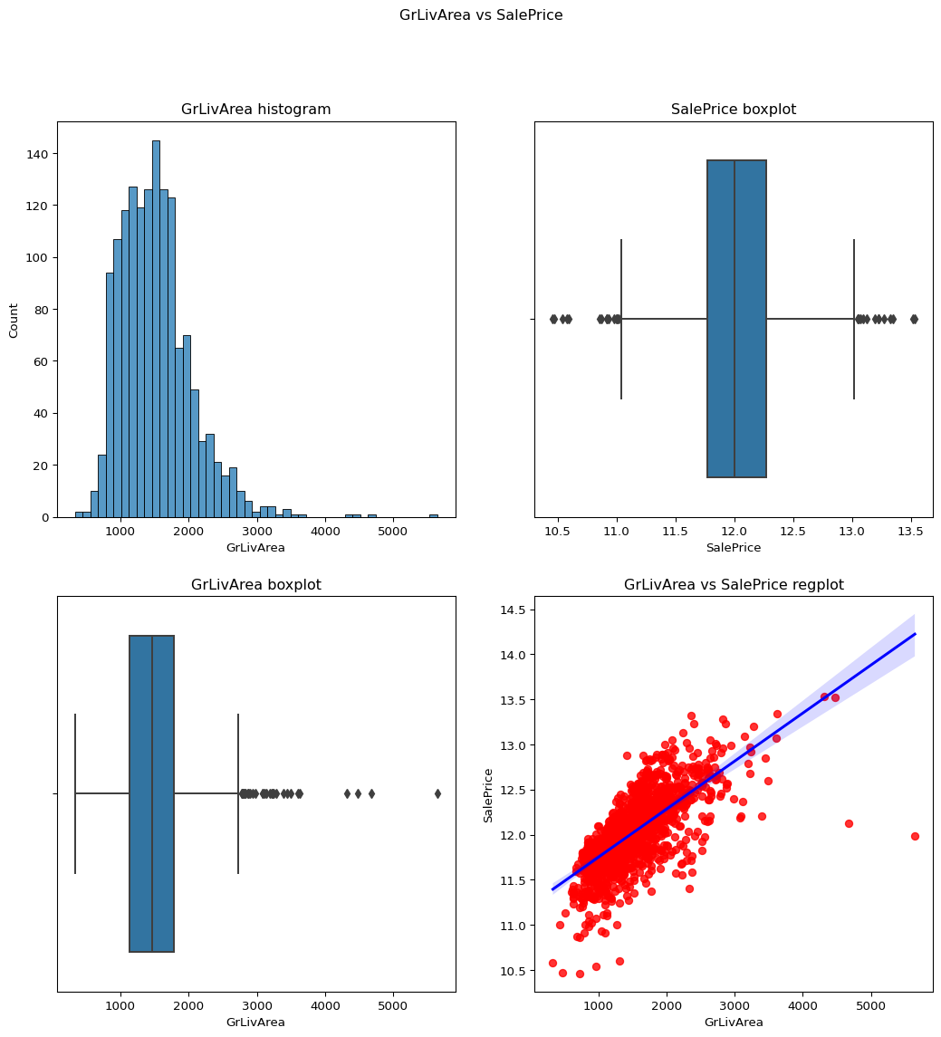
Skewness = 1.3665603560164552.
The skewness of this data is accepable so no need to apply the log transfrom as it would make it negatively skewed.
Code
``` python contvssale(contvar="GrLivArea",df=df) check_column_skewness(df,"GrLivArea") ```1.3665603560164552
FullBath: Full bathrooms above grade
From the regression plot as well as the boxplot we can conclude that the data is not skewed.
It is a descrete variable as well.
Skewness = 0.036561558402727165
Code
``` python check_column_skewness(df,"FullBath") catgvssale(catgvar="FullBath",df=df) ```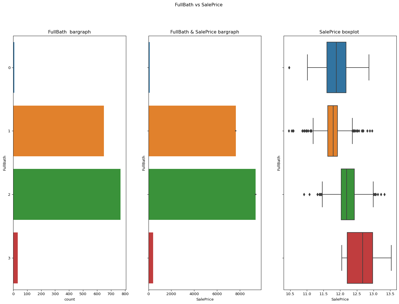
BedroomAbvGr: Bedrooms above grade
It appears as a continuous column but according to its bar graph it is clear that it is descrete.
Code
``` python catgvssale(catgvar="BedroomAbvGr",df=df) ```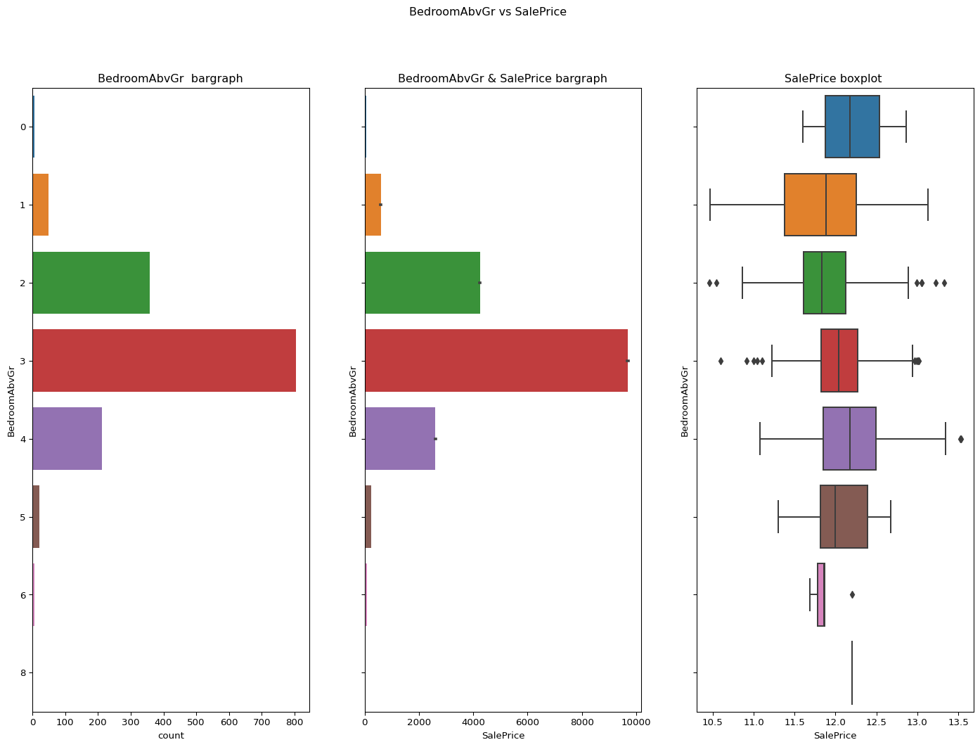
KitchenAbvGr: Kitchens above grade
Code
``` python catgvssale(catgvar="KitchenAbvGr",df=df) ```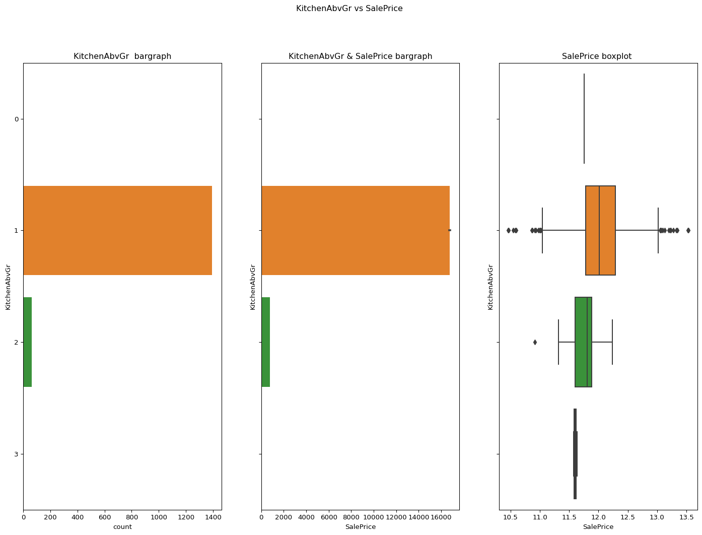
TotRmsAbvGrd: Total rooms above grade (does not include bathrooms)
From the below info we can see that the data is under the skew limit and the graph is normal.
Skewness = 0.6763408364355531
Code
``` python check_column_skewness(df,"TotRmsAbvGrd") catgvssale(catgvar="TotRmsAbvGrd",df=df) ```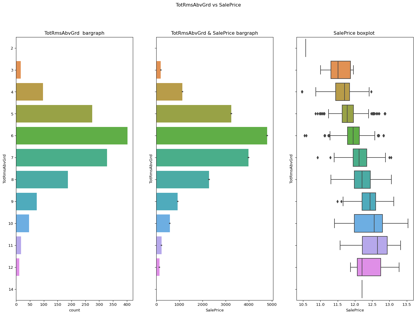
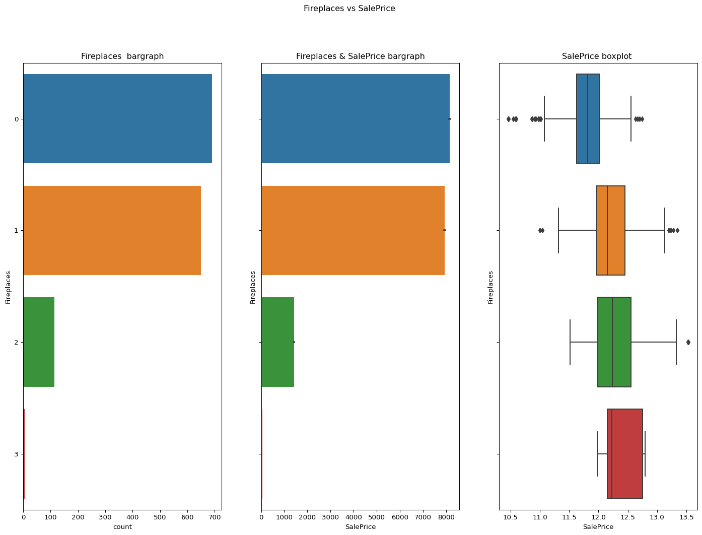
Fireplaces: Number of fireplaces
The data is under the skewness limit of 1.
It can be seen from the graphs as well.
skewness = 0.6495651830548841
Code
``` python contvssale(contvar="Fireplaces",df=df) check_column_skewness(df,"Fireplaces") catgvssale(catgvar="Fireplaces",df=df) ```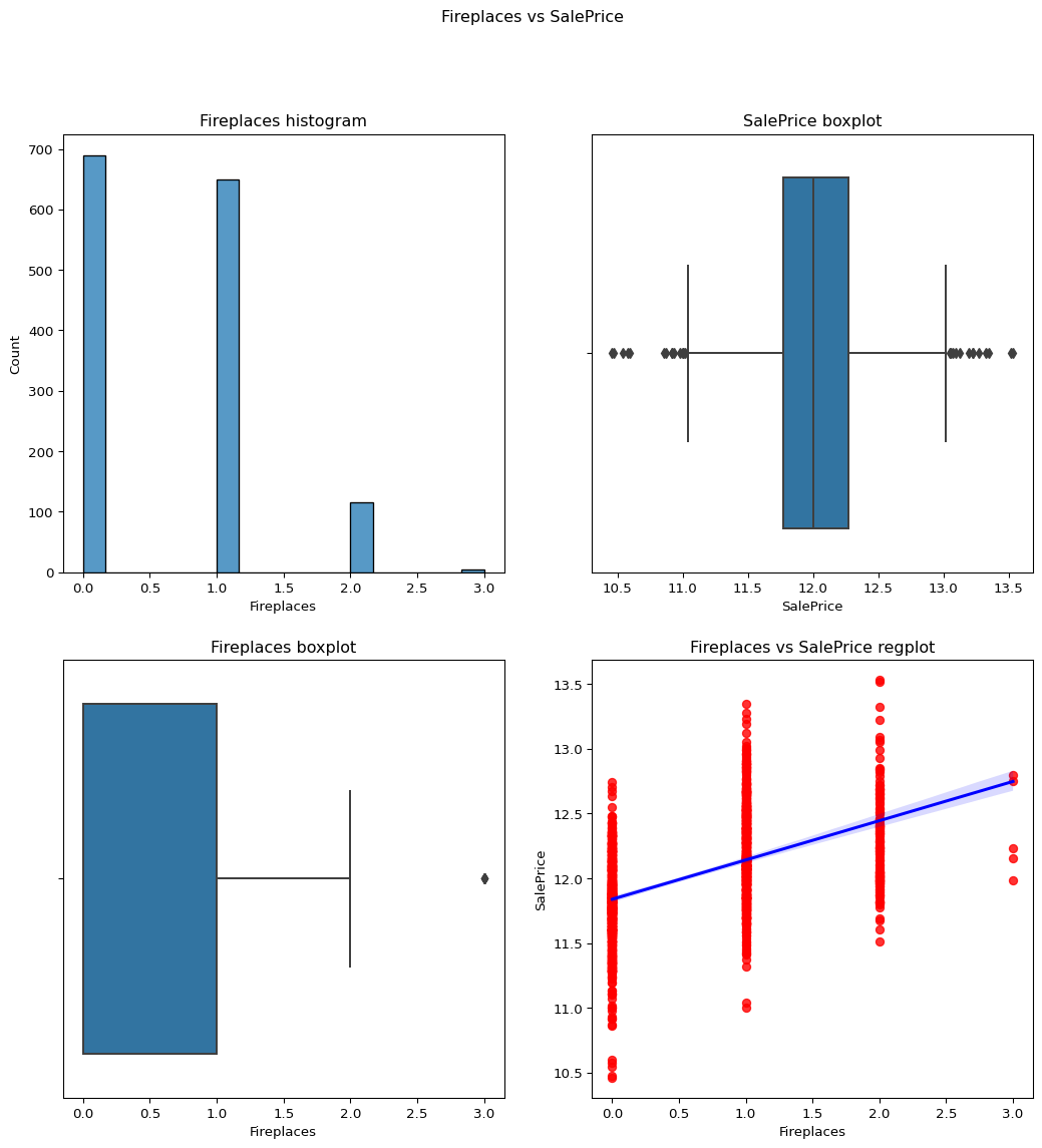
GarageCars: Size of garage in car capacity
From the below visualization it can be predicted that this data column is not skewed its normal.
skewness = -0.3425489297486655
Code
``` python contvssale(contvar="GarageCars",df=df) check_column_skewness(df,"GarageCars") catgvssale(catgvar="GarageCars",df=df) ```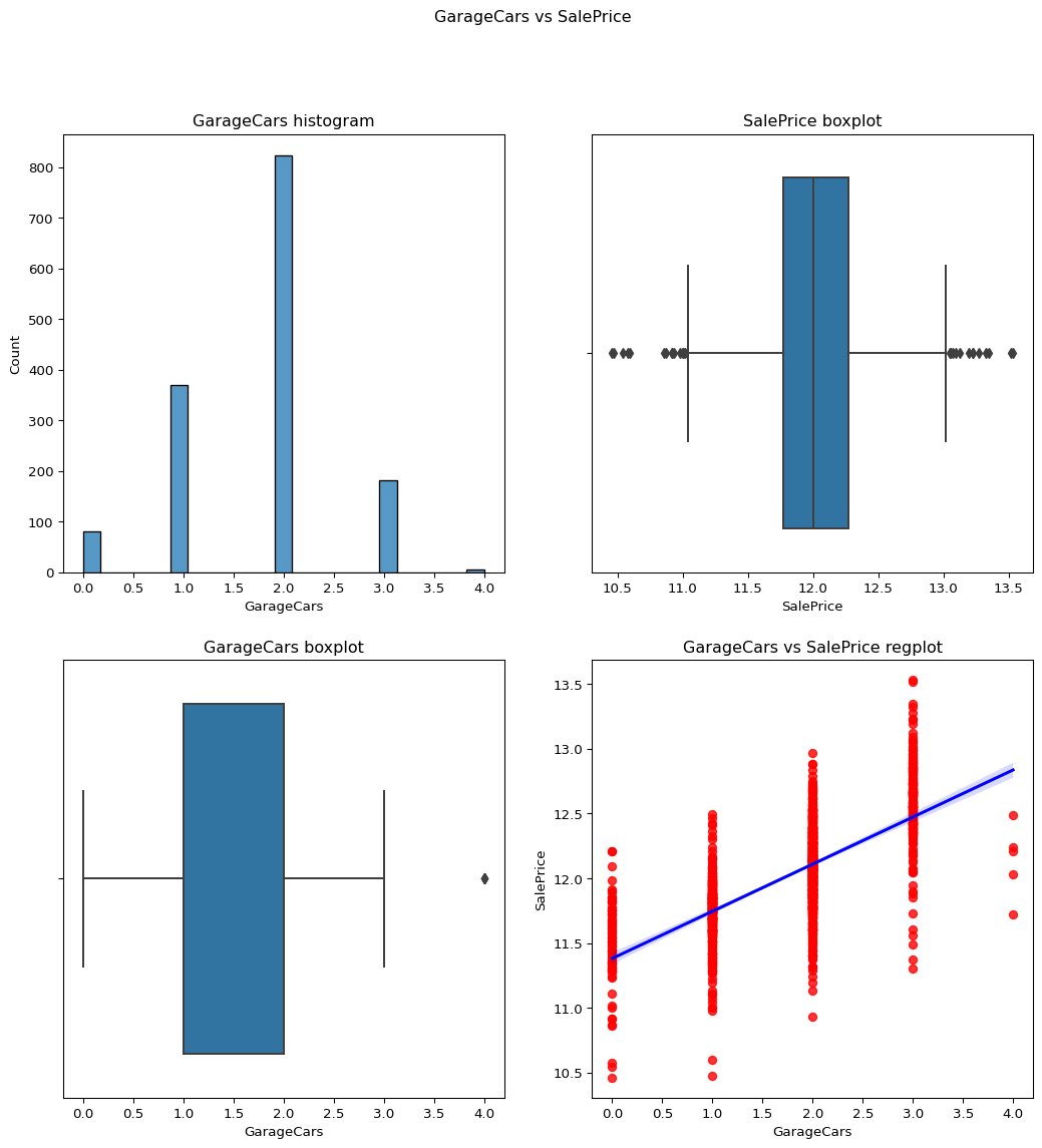
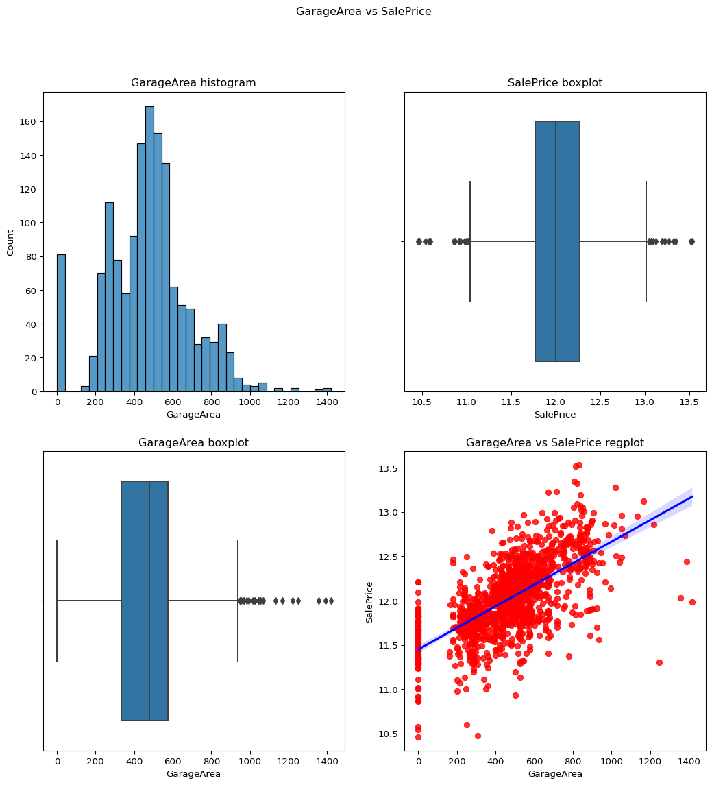
GarageArea: Size of garage in square feet
skewness = 0.17998090674623907
Data column is acceptable.
Code
``` python contvssale(contvar="GarageArea",df=df) check_column_skewness(df,"GarageArea") ```0.17998090674623907
garagecars vs garage area
Code
``` python contvscont(contvar="GarageArea",df=df,tarvar="GarageCars") ```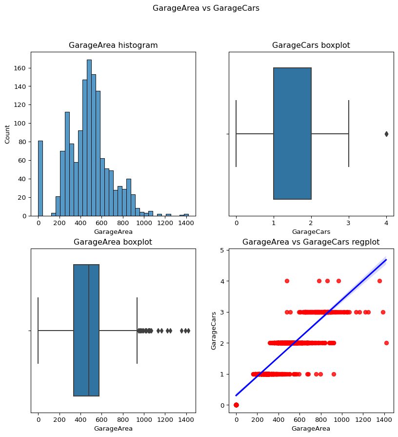
OpenPorchSF: Open porch area in square feet(best)
skewness = 2.3643417403694404
skewness after = -0.02339729485739231
Code
``` python check_column_skewness(df,"OpenPorchSF") remove_skewness(df,"OpenPorchSF") temp_df=temp_df = df.loc[df['OpenPorchSF']!=0] contvssale(contvar="OpenPorchSF",df=temp_df) ```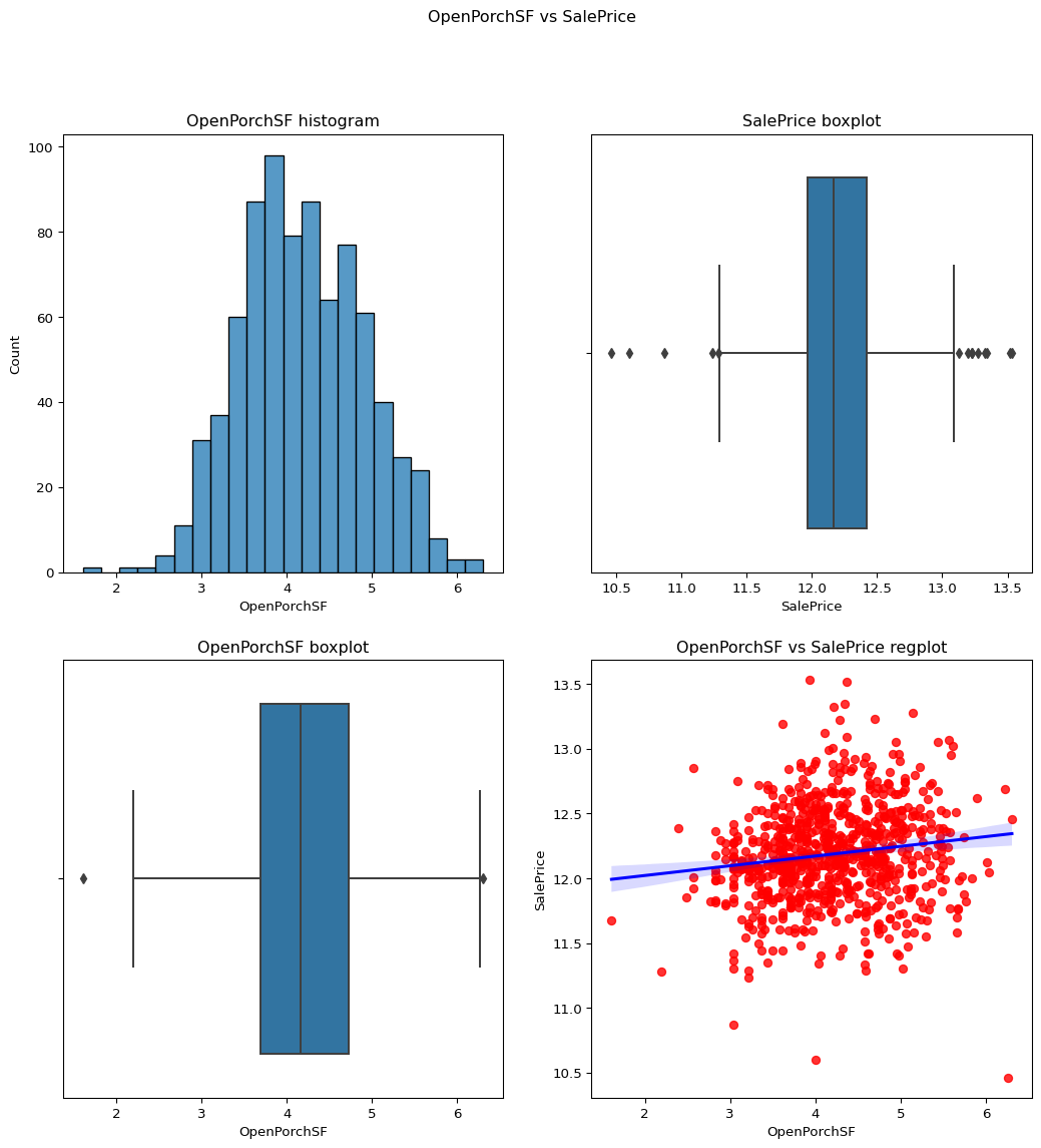
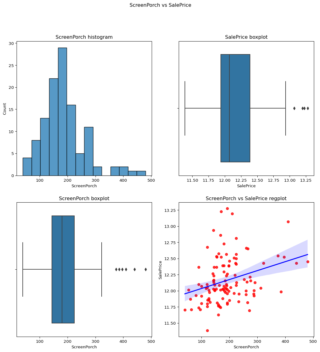
ScreenPorch: Screen porch area in square feet
Skewness before transform = 4.122213743143115
Just after removing the 0 values the skewness came upto 1.186468489847003.
After removing the skewness values of the temp_df we get it -0.40 .
Code
``` python check_column_skewness(df,"ScreenPorch") temp_df=temp_df = df.loc[df['ScreenPorch']!=0] contvssale(contvar="ScreenPorch",df=temp_df) check_column_skewness(temp_df,"ScreenPorch") ```1.186468489847003
current age of the buildings according to the YearRemodAdd
Code
``` python temp_df = df current_year = datetime.now().year temp_df['Age']= current_year-df['YearRemodAdd'] #print(temp_df) temp_df['Age'] contvscont(contvar='Age',df=temp_df,tarvar='SalePrice') ```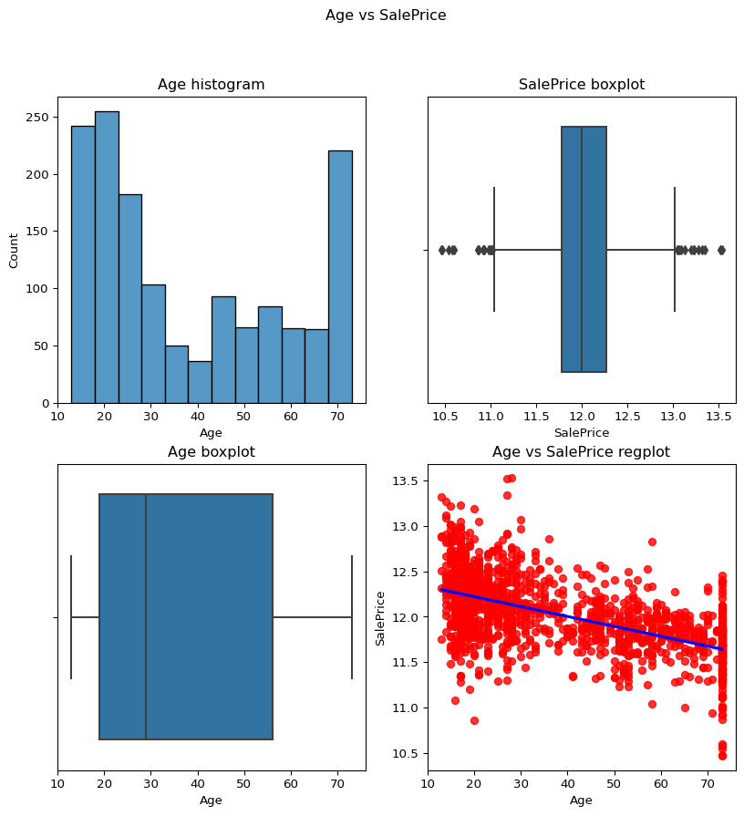
Age of the building acc to the yearsold
Code
``` python temp_df['tempAge']= df['YrSold']-df['YearRemodAdd'] #print(temp_df) temp_df['tempAge'] contvssale(contvar="tempAge",df=temp_df) ```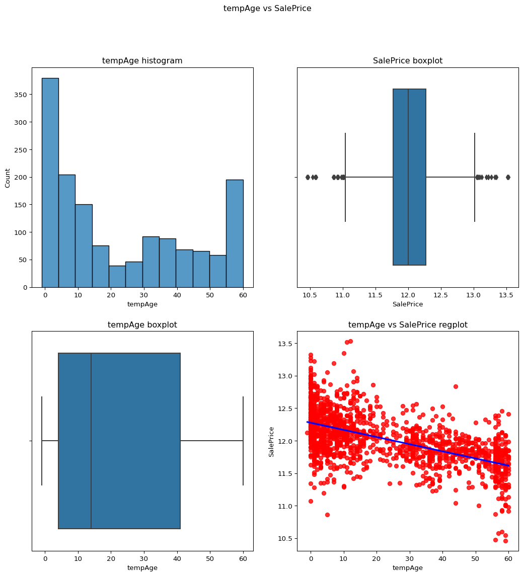
garage year built
Code
``` python temp_df = df current_year = datetime.now().year temp_df['GarAgeYr']= current_year-df['GarageYrBlt'] temp_df['GarAgeYr'] contvssale(contvar='GarAgeYr',df=temp_df) ```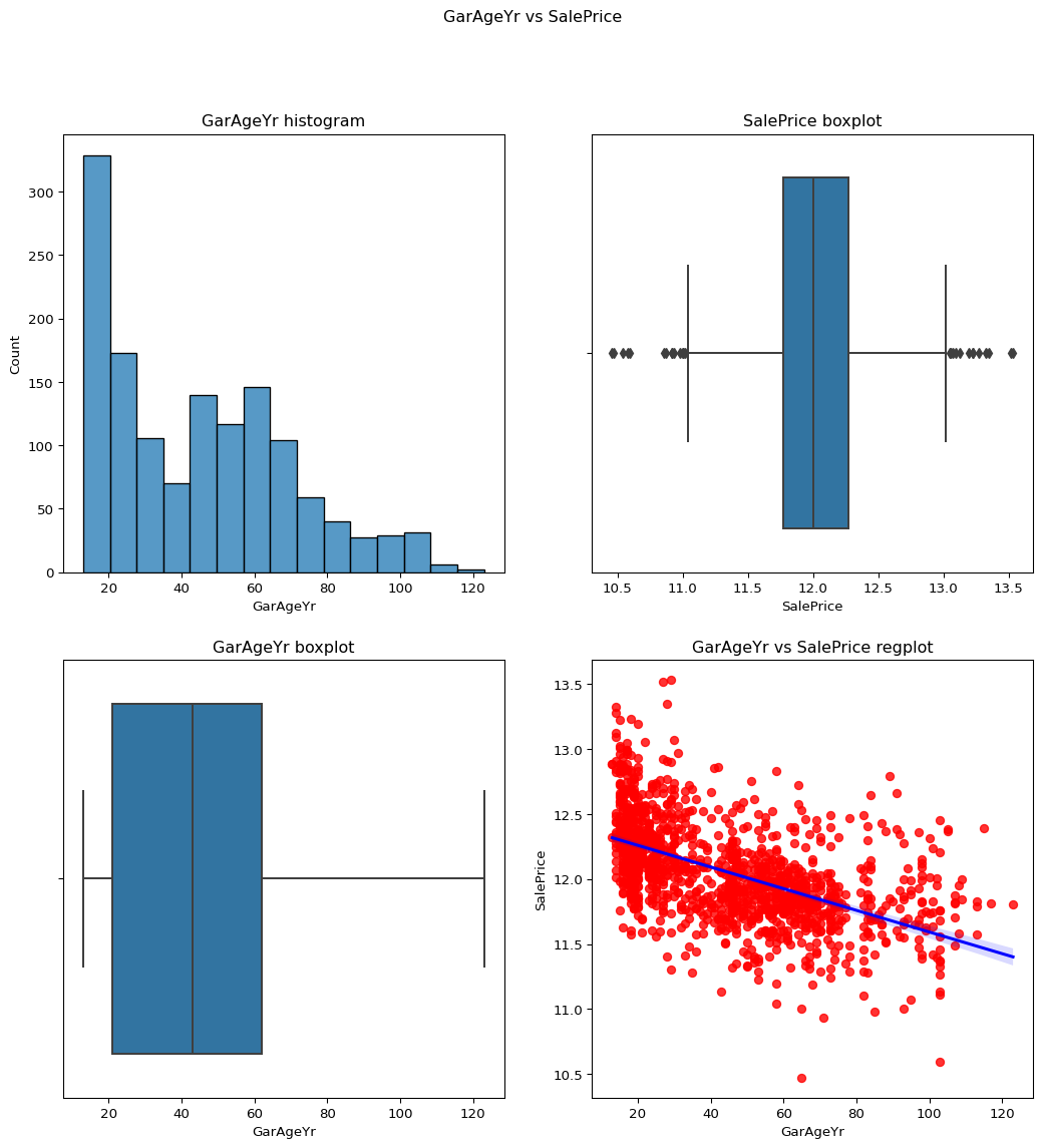
🎯TRAINING AND EVALUATION :
Split the preprocessed dataset into training and testing sets to evaluate the model’s performance on unseen data.Ensure proper stratification if the dataset is imbalanced or if specific classes or categories need to be represented equally in both sets.
Code
``` python import numpy as np import pandas as pd import matplotlib.pyplot as plt import seaborn as sb from sklearn.preprocessing import LabelEncoder from src.util import catgvssale,contvssale,contvscont,check_column_skewness,remove_skewness,plot_contv,remove_ngskewness,preprocess_dataset from datetime import datetime from scipy.stats import skew from sklearn.linear_model import Lasso from sklearn.preprocessing import StandardScaler from sklearn.feature_selection import SelectPercentile, chi2 from sklearn.linear_model import LinearRegression from sklearn.metrics import r2_score from sklearn.metrics import mean_squared_error import pickle ```Code
``` python final_df = pd.read_csv('data/raw/train.csv') df1 = pd.read_csv('data/raw/train.csv') lbl_dsc = pd.read_csv('data\clean\label_description.csv') var_dsc = pd.read_csv('data/clean/variable_description.csv') ```Select the variables that are Nominal from var_dsc
From the variable description file we are collecting only the variables that are nominal so that we can add it to the list of nominal data.
Code
``` python nominal_df = var_dsc.loc[var_dsc['variable_type'] == 'Nominal'] #print(ordinal_df) #nominal_df.head(30) nominal_list = nominal_df['variable'].to_list() print(nominal_list) nominal_list.remove("MiscFeature") nominal_list.remove("Alley") nominal_list.remove("MSSubClass") print(nominal_list) ```['MSSubClass', 'MSZoning', 'Street', 'Alley', 'LandContour', 'LotConfig', 'Neighborhood', 'Condition1', 'Condition2', 'BldgType', 'HouseStyle', 'RoofStyle', 'RoofMatl', 'Exterior1st', 'Exterior2nd', 'MasVnrType', 'Foundation', 'Heating', 'CentralAir', 'GarageType', 'MiscFeature', 'SaleType', 'SaleCondition']
['MSZoning', 'Street', 'LandContour', 'LotConfig', 'Neighborhood', 'Condition1', 'Condition2', 'BldgType', 'HouseStyle', 'RoofStyle', 'RoofMatl', 'Exterior1st', 'Exterior2nd', 'MasVnrType', 'Foundation', 'Heating', 'CentralAir', 'GarageType', 'SaleType', 'SaleCondition']
Select the variables that are Ordinal from var_dsc
From the variable description file we are collecting only the variables that are ordinal so that we can add it to the list of ordinal data.
Code
``` python ordinal_df = var_dsc.loc[var_dsc['variable_type'] == 'Ordinal'] #print(ordinal_df) ordinal_df.head(24) ordinal_list = ordinal_df['variable'].to_list() print(ordinal_list) ordinal_list.remove("PoolQC") ordinal_list.remove("Fence") print(ordinal_list) ```['LotShape', 'Utilities', 'LandSlope', 'OverallQual', 'OverallCond', 'ExterQual', 'ExterCond', 'BsmtQual', 'BsmtCond', 'BsmtExposure', 'BsmtFinType1', 'BsmtFinType2', 'HeatingQC', 'Electrical', 'KitchenQual', 'Functional', 'FireplaceQu', 'GarageFinish', 'GarageQual', 'GarageCond', 'PavedDrive', 'PoolQC', 'Fence']
['LotShape', 'Utilities', 'LandSlope', 'OverallQual', 'OverallCond', 'ExterQual', 'ExterCond', 'BsmtQual', 'BsmtCond', 'BsmtExposure', 'BsmtFinType1', 'BsmtFinType2', 'HeatingQC', 'Electrical', 'KitchenQual', 'Functional', 'FireplaceQu', 'GarageFinish', 'GarageQual', 'GarageCond', 'PavedDrive']
Select the variables that are Continuous from var_dsc
From the variable description file we are collecting only the variables that are continuous so that we can add it to the list of continuous data.
Code
``` python cont_df = var_dsc.loc[var_dsc['variable_type'] == 'Continuous'] cont_list = cont_df['variable'].to_list() print(cont_list) ```['LotFrontage', 'LotArea', 'MasVnrArea', 'BsmtFinSF1', 'BsmtFinSF2', 'BsmtUnfSF', 'TotalBsmtSF', '1stFlrSF', '2ndFlrSF', 'LowQualFinSF', 'GrLivArea', 'GarageArea', 'WoodDeckSF', 'OpenPorchSF', 'EnclosedPorch', '3SsnPorch', 'ScreenPorch', 'PoolArea', 'MiscVal', 'SalePrice']
Creating arguments for the function to be used
Code
``` python ordinal_vars = ordinal_list continuous_vars = cont_list nominal_vars = nominal_list ```Dropping the columns with the most missing ratio
Code
``` python df1 = df1.drop(['Alley','PoolQC','MiscFeature','Fence'],axis=1) df1.fillna(0) print('Dropped columns are : Alley,PoolQC,MiscFeature,Fence') ```Dropped columns are : Alley,PoolQC,MiscFeature,Fence
Applying labelencoding , one hot encoding and log tranfromation on the above generated lists
We apply labelencoding for the ordinal variables, one hot encoding for the nominal variables and log transformation for the continuous variables.
Code
``` python def preprocess_dataset(dataset, continuous_vars, nominal_vars, ordinal_vars): print(dataset.shape) transformed_dataset = log_transform_continuous(dataset, continuous_vars) print(transformed_dataset.shape) encoded_dataset = one_hot_encode_nominal(transformed_dataset, nominal_vars) print(encoded_dataset.shape) preprocessed_dataset = label_encode_dataset(encoded_dataset, ordinal_vars) print(preprocessed_dataset.shape) return preprocessed_dataset final_data = preprocess_dataset(df1, continuous_vars, nominal_vars, ordinal_vars) ```(1460, 77)
(1460, 77)
(1460, 191)
(1460, 191)
Splitting the data
Code
``` python columnindex = final_data.columns.get_loc('SalePrice') print(columnindex) X1 = final_data.iloc[:,0:columnindex] y = final_data.iloc[:,columnindex] X2 = final_data.iloc[:,(columnindex + 1):192] X = pd.concat([X1,X2],axis=1) X = X.fillna(0) X.drop('Id',axis=1) X ```56
1460 rows × 190 columns
MODEL 1 :
Linear Regression Model With the Mutual Information Data
Code
``` python from sklearn.linear_model import LinearRegression from sklearn.feature_selection import SelectKBest, mutual_info_regression from sklearn.model_selection import train_test_split # Split the data into features (X) and target variable (y) # Apply SelectKBest feature selection k = 170 # Number of top features to select selector = SelectKBest(score_func=mutual_info_regression, k=k) X_selected = selector.fit_transform(X, y) X_train, X_test, y_train, y_test = train_test_split(X_selected, y, test_size=0.3, random_state=42) # Get selected feature names #selected_feature_names = X.columns[selector.get_support()].tolist() # Fit a linear regression model using the selected features linear_regression = LinearRegression() linear_regression.fit(X_train, y_train) y_pred = linear_regression.predict(X_test) y_predsp = np.expm1(y_pred) y_testsp = np.expm1(y_test) ```Scores
Code
``` python mse = mean_squared_error(y_testsp, y_predsp) r2 = r2_score(y_testsp, y_predsp) rmse = mean_squared_error(y_testsp, y_predsp,squared=False) print("Mean Squared Error (RMSE) on train set:", mse) print("Root Mean Squared Error (MSE) on train set:", rmse) print("R-squared score on train set:", r2) le = round(linear_regression.score(X_test,y_test), 2) print(le) ```Mean Squared Error (RMSE) on train set: 551468179.5154297
Root Mean Squared Error (MSE) on train set: 23483.35963007486
R-squared score on train set: 0.9209715147993085
0.91
MODEL 2 :
RandomForest Regression
Code
``` python from sklearn.ensemble import RandomForestRegressor X_train, X_test, y_train, y_test = train_test_split(X_selected, y, test_size=0.3, random_state=42) # create regressor object regressor = RandomForestRegressor(n_estimators=100,random_state=0,oob_score=True) # fit the regressor with x and y data regressor.fit(X_train, y_train) Y_pred = regressor.predict(X_test) Y_predsp = np.expm1(Y_pred) Y_testsp = np.expm1(y_test) ```Scores of the RandomForest Regression
Code
``` python print(regressor.oob_score_) r2 = r2_score(Y_testsp, Y_predsp) rmse = mean_squared_error(Y_testsp, Y_predsp,squared=False) print("R-squared score on train set:", r2) print("Root Mean Squared Error (MSE) on train set:", rmse) ```0.8558424487348482
R-squared score on train set: 0.8889903973831512
Root Mean Squared Error (MSE) on train set: 27832.272911585656
➡️CONCLUSION :
From the above insights on the various scores and rmse and r2 values we can conclude that linear regression model with the mutual information data will be the most suitable for this house price prediction model.